Handbook of Regression Modeling in People Analytics: With Examples in R and Python

Keith McNulty

7 Proportional Odds Logistic Regression for Ordered Category Outcomes

Often our outcomes will be categorical in nature, but they will also have an order to them. These are sometimes known as ordinal outcomes. Some very common examples of this include ratings of some form, such as job performance ratings or survey responses on Likert scales. The appropriate modeling approach for these outcome types is ordinal logistic regression. Surprisingly, this approach is frequently not understood or adopted by analysts. Often they treat the outcome as a continuous variable and perform simple linear regression, which can lead to wildly inaccurate inferences. Given the prevalence of ordinal outcomes in people analytics, it would serve analysts well to know how to run ordinal logistic regression models, how to interpret them and how to confirm their validity.

In fact, there are numerous known ways to approach the inferential modeling of ordinal outcomes, all of which build on the theory of linear, binomial and multinomial regression which we covered in previous chapters. In this chapter, we will focus on the most commonly adopted approach: proportional odds logistic regression. Proportional odds models (sometimes known as constrained cumulative logistic models) are more attractive than other approaches because of their ease of interpretation but cannot be used blindly without important checking of underlying assumptions.

7.1 When to use it

7.1.1 Intuition for proportional odds logistic regression

Ordinal outcomes can be considered to be suitable for an approach somewhere ‘between’ linear regression and multinomial regression. In common with linear regression, we can consider our outcome to increase or decrease dependent on our inputs. However, unlike linear regression the increase and decrease is ‘stepwise’ rather than continuous, and we do not know that the difference between the steps is the same across the scale. In medical settings, the difference between moving from a healthy to an early-stage disease may not be equivalent to moving from an early-stage disease to an intermediate- or advanced-stage. Equally, it may be a much bigger psychological step for an individual to say that they are very dissatisfied in their work than it is to say that they are very satisfied in their work. In this sense, we are analyzing categorical outcomes similar to a multinomial approach.

To formalize this intuition, we can imagine a latent version of our outcome variable that takes a continuous form, and where the categories are formed at specific cutoff points on that continuous variable. For example, if our outcome variable \(y\) represents survey responses on an ordinal Likert scale of 1 to 5, we can imagine we are actually dealing with a continuous variable \(y'\) along with four increasing ‘cutoff points’ for \(y'\) at \(\tau_1\), \(\tau_2\), \(\tau_3\) and \(\tau_4\). We then define each ordinal category as follows: \(y = 1\) corresponds to \(y' \le \tau_1\), \(y \le 2\) to \(y' \le \tau_2\), \(y \le 3\) to \(y' \le \tau_3\) and \(y \le 4\) to \(y' \le \tau_4\). Further, at each such cutoff \(\tau_k\), we assume that the probability \(P(y > \tau_k)\) takes the form of a logistic function. Therefore, in the proportional odds model, we ‘divide’ the probability space at each level of the outcome variable and consider each as a binomial logistic regression model. For example, at rating 3, we generate a binomial logistic regression model of \(P(y > \tau_3)\), as illustrated in Figure 7.1.

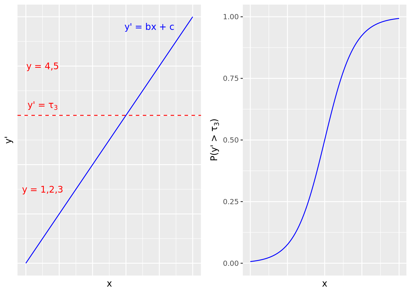
Proportional odds model illustration for a 5-point Likert survey scale outcome greater than 3 on a single input variable. Each cutoff point in the latent continuous outcome variable gives rise to a binomial logistic function.

Figure 7.1: Proportional odds model illustration for a 5-point Likert survey scale outcome greater than 3 on a single input variable. Each cutoff point in the latent continuous outcome variable gives rise to a binomial logistic function.

This approach leads to a highly interpretable model that provides a single set of coefficients that are agnostic to the outcome category. For example, we can say that each unit increase in input variable \(x\) increases the odds of \(y\) being in a higher category by a certain ratio.

7.1.2 Use cases for proportional odds logistic regression

Proportional odds logistic regression can be used when there are more than two outcome categories that have an order. An important underlying assumption is that no input variable has a disproportionate effect on a specific level of the outcome variable. This is known as the proportional odds assumption. Referring to Figure 7.1, this assumption means that the ‘slope’ of the logistic function is the same for all category cutoffs³⁴. If this assumption is violated, we cannot reduce the coefficients of the model to a single set across all outcome categories, and this modeling approach fails. Therefore, testing the proportional odds assumption is an important validation step for anyone running this type of model.

Examples of problems that can utilize a proportional odds logistic regression approach include:

Understanding the factors associated with higher ratings in an employee survey on a Likert scale
Understanding the factors associated with higher job performance ratings on an ordinal performance scale
Understanding the factors associated with voting preference in a ranked preference voting system (for example, proportional representation systems)

7.1.3 Walkthrough example

You are an analyst for a sports broadcaster who is doing a feature on player discipline in professional soccer games. To prepare for the feature, you have been asked to verify whether certain metrics are significant in influencing the extent to which a player will be disciplined by the referee for unfair or dangerous play in a game. You have been provided with data on over 2000 different players in different games, and the data contains these fields:

discipline: A record of the maximum discipline taken by the referee against the player in the game. ‘None’ means no discipline was taken, ‘Yellow’ means the player was issued a yellow card (warned), ‘Red’ means the player was issued a red card and ordered off the field of play.
n_yellow_25 is the total number of yellow cards issued to the player in the previous 25 games they played prior to this game.
n_red_25 is the total number of red cards issued to the player in the previous 25 games they played prior to this game.
position is the playing position of the player in the game: ‘D’ is defense (including goalkeeper), ‘M’ is midfield and ‘S’ is striker/attacker.
level is the skill level of the competition in which the game took place, with 1 being higher and 2 being lower.
country is the country in which the game took place—England or Germany.
result is the result of the game for the team of the player—‘W’ is win, ‘L’ is lose, ‘D’ is a draw/tie.

Let’s download the soccer data set and take a quick look at it.

# if needed, download data
url <- "http://peopleanalytics-regression-book.org/data/soccer.csv"
soccer <- read.csv(url)

head(soccer)

##   discipline n_yellow_25 n_red_25 position result country level
## 1       None           4        1        S      D England     1
## 2       None           2        2        D      W England     2
## 3       None           2        1        M      D England     1
## 4       None           2        1        M      L Germany     1
## 5       None           2        0        S      W Germany     1
## 6       None           3        2        M      W England     1

Let’s also take a look at the structure of the data.

str(soccer)

## 'data.frame':    2291 obs. of  7 variables:
##  $ discipline : chr  "None" "None" "None" "None" ...
##  $ n_yellow_25: int  4 2 2 2 2 3 4 3 4 3 ...
##  $ n_red_25   : int  1 2 1 1 0 2 2 0 3 3 ...
##  $ position   : chr  "S" "D" "M" "M" ...
##  $ result     : chr  "D" "W" "D" "L" ...
##  $ country    : chr  "England" "England" "England" "Germany" ...
##  $ level      : int  1 2 1 1 1 1 2 1 1 1 ...

We see that there are numerous fields that need to be converted to factors before we can model them. Firstly, our outcome of interest is discipline and this needs to be an ordered factor, which we can choose to increase with the seriousness of the disciplinary action.

# convert discipline to ordered factor
soccer$discipline <- ordered(soccer$discipline, 
                             levels = c("None", "Yellow", "Red"))

# check conversion
str(soccer)

## 'data.frame':    2291 obs. of  7 variables:
##  $ discipline : Ord.factor w/ 3 levels "None"<"Yellow"<..: 1 1 1 1 1 1 1 1 1 1 ...
##  $ n_yellow_25: int  4 2 2 2 2 3 4 3 4 3 ...
##  $ n_red_25   : int  1 2 1 1 0 2 2 0 3 3 ...
##  $ position   : chr  "S" "D" "M" "M" ...
##  $ result     : chr  "D" "W" "D" "L" ...
##  $ country    : chr  "England" "England" "England" "Germany" ...
##  $ level      : int  1 2 1 1 1 1 2 1 1 1 ...

We also know that position, country, result and level are categorical, so we convert them to factors. We could in fact choose to convert result and level into ordered factors if we so wish, but this is not necessary for input variables, and the results are usually a little bit easier to read as nominal factors.

# apply as.factor to four columns
cats <- c("position", "country", "result", "level")
soccer[ ,cats] <- lapply(soccer[ ,cats], as.factor)

# check again
str(soccer)

## 'data.frame':    2291 obs. of  7 variables:
##  $ discipline : Ord.factor w/ 3 levels "None"<"Yellow"<..: 1 1 1 1 1 1 1 1 1 1 ...
##  $ n_yellow_25: int  4 2 2 2 2 3 4 3 4 3 ...
##  $ n_red_25   : int  1 2 1 1 0 2 2 0 3 3 ...
##  $ position   : Factor w/ 3 levels "D","M","S": 3 1 2 2 3 2 2 2 2 1 ...
##  $ result     : Factor w/ 3 levels "D","L","W": 1 3 1 2 3 3 3 3 1 2 ...
##  $ country    : Factor w/ 2 levels "England","Germany": 1 1 1 2 2 1 2 1 2 1 ...
##  $ level      : Factor w/ 2 levels "1","2": 1 2 1 1 1 1 2 1 1 1 ...

Now our data is in a position to run a model. You may wish to conduct some exploratory data analysis at this stage similar to previous chapters, but from this chapter onward we will skip this and focus on the modeling methodology.

7.2 Modeling ordinal outcomes under the assumption of proportional odds

For simplicity, and noting that this is easily generalizable, let’s assume that we have an ordinal outcome variable \(y\) with three levels similar to our walkthrough example, and that we have one input variable \(x\). Let’s call the outcome levels 1, 2 and 3. To follow our intuition from Section 7.1.1, we can model a linear continuous variable \(y' = \alpha_1x + \alpha_0 + E\), where \(E\) is some error with a mean of zero, and two increasing cutoff values \(\tau_1\) and \(\tau_2\). We define \(y\) in terms of \(y'\) as follows: \(y = 1\) if \(y' \le \tau_1\), \(y = 2\) if \(\tau_1 < y' \le \tau_2\) and \(y = 3\) if \(y' > \tau_2\).

7.2.1 Using a latent continuous outcome variable to derive a proportional odds model

Recall from Section 4.5.3 that our linear regression approach assumes that our residuals \(E\) around our line \(y' = \alpha_1x + \alpha_0\) have a normal distribution. Let’s modify that assumption slightly and instead assume that our residuals take a logistic distribution based on the variance of \(y'\). Therefore, \(y' = \alpha_1x + \alpha_0 + \sigma\epsilon\), where \(\sigma\) is proportional to the variance of \(y'\) and \(\epsilon\) follows the shape of a logistic function. That is

\[ P(\epsilon \leq z) = \frac{1}{1 + e^{-z}} \]

Let’s look at the probability that our ordinal outcome variable \(y\) is in its lowest category.

\[ \begin{aligned} P(y = 1) &= P(y' \le \tau_1) \\ &= P(\alpha_1x + \alpha_0 + \sigma\epsilon \leq \tau_1) \\ &= P(\epsilon \leq \frac{\tau_1 - \alpha_1x - \alpha_0}{\sigma}) \\ &= P(\epsilon \le \gamma_1 - \beta{x}) \\ &= \frac{1}{1 + e^{-(\gamma_1 - \beta{x})}} \end{aligned} \]

where \(\gamma_1 = \frac{\tau_1 - \alpha_0}{\sigma}\) and \(\beta = \frac{\alpha_1}{\sigma}\).

Since our only values for \(y\) are 1, 2 and 3, similar to our derivations in Section 5.2, we conclude that \(P(y > 1) = 1 - P(y = 1)\), which calculates to

\[ P(y > 1) = \frac{e^{-(\gamma_1 - \beta{x})}}{1 + e^{-(\gamma_1 - \beta{x})}} \] Therefore \[ \begin{aligned} \frac{P(y = 1)}{P(y > 1)} = \frac{\frac{1}{1 + e^{-(\gamma_1 - \beta{x})}}}{\frac{e^{-(\gamma_1 - \beta{x})}}{1 + e^{-(\gamma_1 - \beta{x})}}} = e^{\gamma_1 - \beta{x}} \end{aligned} \]

By applying the natural logarithm, we conclude that the log odds of \(y\) being in our bottom category is

\[ \mathrm{ln}\left(\frac{P(y = 1)}{P(y > 1)}\right) = \gamma_1 - \beta{x} \] In a similar way we can derive the log odds of our ordinal outcome being in our bottom two categories as

\[ \mathrm{ln}\left(\frac{P(y \leq 2)}{P(y = 3)}\right) = \gamma_2 - \beta{x} \] where \(\gamma_2 = \frac{\tau_2 - \alpha_0}{\sigma}\). One can easily see how this generalizes to an arbitrary number of ordinal categories, where we can state the log odds of being in category \(k\) or lower as

\[ \mathrm{ln}\left(\frac{P(y \leq k)}{P(y > k)}\right) = \gamma_k - \beta{x} \] Alternatively, we can state the log odds of being in a category higher than \(k\) by simply inverting the above expression:

\[ \mathrm{ln}\left(\frac{P(y > k)}{P(y \leq k)}\right) = -(\gamma_k - \beta{x}) = \beta{x} - \gamma_k \]

By taking exponents we see that the impact of a unit change in \(x\) on the odds of \(y\) being in a higher ordinal category is \(\beta\), irrespective of what category we are looking at. Therefore we have a single coefficient to explain the effect of \(x\) on \(y\) throughout the ordinal scale. Note that there are still different intercept coefficients \(\gamma_1\) and \(\gamma_2\) for each level of the ordinal scale.

7.2.2 Running a proportional odds logistic regression model

The MASS package provides a function polr() for running a proportional odds logistic regression model on a data set in a similar way to our previous models. The key (and obvious) requirement is that the outcome is an ordered factor. Since we did our conversions in Section 7.1.3 we are ready to run this model. We will start by running it on all input variables and let the polr() function handle our dummy variables automatically.

# run proportional odds model
library(MASS)
model <- polr(
  formula = discipline ~ n_yellow_25 + n_red_25 + position + 
    country + level + result, 
  data = soccer
)

# get summary
summary(model)

## Call:
## polr(formula = discipline ~ n_yellow_25 + n_red_25 + position + 
##     country + level + result, data = soccer)
## 
## Coefficients:
##                   Value Std. Error t value
## n_yellow_25     0.32236    0.03308  9.7456
## n_red_25        0.38324    0.04051  9.4616
## positionM       0.19685    0.11649  1.6899
## positionS      -0.68534    0.15011 -4.5655
## countryGermany  0.13297    0.09360  1.4206
## level2          0.09097    0.09355  0.9724
## resultL         0.48303    0.11195  4.3147
## resultW        -0.73947    0.12129 -6.0966
## 
## Intercepts:
##             Value   Std. Error t value
## None|Yellow  2.5085  0.1918    13.0770
## Yellow|Red   3.9257  0.2057    19.0834
## 
## Residual Deviance: 3444.534 
## AIC: 3464.534

We can see that the summary returns a single set of coefficients on our input variables as we expect, with standard errors and t-statistics. We also see that there are separate intercepts for the various levels of our outcomes, as we also expect. In interpreting our model, we generally don’t have a great deal of interest in the intercepts, but we will focus on the coefficients. First we would like to obtain p-values, so we can add a p-value column using the conversion methods from the t-statistic which we learned in Section 3.3.1 ³⁵.

# get coefficients (it's in matrix form)
coefficients <- summary(model)$coefficients

# calculate p-values
p_value <- (1 - pnorm(abs(coefficients[ ,"t value"]), 0, 1))*2

# bind back to coefficients
(coefficients <- cbind(coefficients, p_value))

##                      Value Std. Error    t value      p_value
## n_yellow_25     0.32236030 0.03307768  9.7455529 0.000000e+00
## n_red_25        0.38324333 0.04050515  9.4615947 0.000000e+00
## positionM       0.19684666 0.11648690  1.6898610 9.105456e-02
## positionS      -0.68533697 0.15011194 -4.5655060 4.982908e-06
## countryGermany  0.13297173 0.09359946  1.4206464 1.554196e-01
## level2          0.09096627 0.09354717  0.9724108 3.308462e-01
## resultL         0.48303227 0.11195131  4.3146639 1.598459e-05
## resultW        -0.73947295 0.12129301 -6.0965834 1.083595e-09
## None|Yellow     2.50850778 0.19182628 13.0769766 0.000000e+00
## Yellow|Red      3.92572124 0.20571423 19.0833721 0.000000e+00

Next we can convert our coefficients to odds ratios.

# calculate odds ratios
odds_ratio <- exp(coefficients[ ,"Value"])

We can display all our critical statistics by combining them into a dataframe.

# combine with coefficient and p_value
(coefficients <- cbind(
  coefficients[ ,c("Value", "p_value")],
  odds_ratio
))

##                      Value      p_value odds_ratio
## n_yellow_25     0.32236030 0.000000e+00  1.3803820
## n_red_25        0.38324333 0.000000e+00  1.4670350
## positionM       0.19684666 9.105456e-02  1.2175573
## positionS      -0.68533697 4.982908e-06  0.5039204
## countryGermany  0.13297173 1.554196e-01  1.1422177
## level2          0.09096627 3.308462e-01  1.0952321
## resultL         0.48303227 1.598459e-05  1.6209822
## resultW        -0.73947295 1.083595e-09  0.4773654
## None|Yellow     2.50850778 0.000000e+00 12.2865822
## Yellow|Red      3.92572124 0.000000e+00 50.6896241

Taking into consideration the p-values, we can interpret our coefficients as follows, in each case assuming that other coefficients are held still:

Each additional yellow card received in the prior 25 games is associated with an approximately 38% higher odds of greater disciplinary action by the referee.
Each additional red card received in the prior 25 games is associated with an approximately 47% higher odds of greater disciplinary action by the referee.
Strikers have approximately 50% lower odds of greater disciplinary action from referees compared to Defenders.
A player on a team that lost the game has approximately 62% higher odds of greater disciplinary action versus a player on a team that drew the game.
A player on a team that won the game has approximately 52% lower odds of greater disciplinary action versus a player on a team that drew the game.

We can, as per previous chapters, remove the level and country variables from this model to simplify it if we wish. An examination of the coefficients and the AIC of the simpler model will reveal no substantial difference, and therefore we proceed with this model.

7.2.3 Calculating the likelihood of an observation being in a specific ordinal category

Recall from Section 7.2.1 that our proportional odds model generates multiple stratified binomial models, each of which has following form:

\[ P(y \leq k) = P(y' \leq \tau_k) \] Note that for an ordinal variable \(y\), if \(y \leq k\) and \(y > k-1\), then \(y = k\). Therefore \(P(y = k) = P(y \leq k) - P(y \leq k - 1)\). This means we can calculate the specific probability of an observation being in each level of the ordinal variable in our fitted model by simply calculating the difference between the fitted values from each pair of adjacent stratified binomial models. In our walkthrough example, this means we can calculate the specific probability of no action from the referee, or a yellow card being awarded, or a red card being awarded. These can be viewed using the fitted() function.

head(fitted(model))

##        None     Yellow        Red
## 1 0.8207093 0.12900184 0.05028889
## 2 0.8514232 0.10799553 0.04058128
## 3 0.7830785 0.15400189 0.06291964
## 4 0.6609864 0.22844107 0.11057249
## 5 0.9591298 0.03064719 0.01022301
## 6 0.7887766 0.15027145 0.06095200

It can be seen from this output how ordinal logistic regression models can be used in predictive analytics by classifying new observations into the ordinal category with the highest fitted probability. This also allows us to graphically understand the output of a proportional odds model. Interactive Figure 7.2 shows the output from a simpler proportional odds model fitted against the n_yellow_25 and n_red_25 input variables, with the fitted probabilities of each level of discipline from the referee plotted on the different colored surfaces. We can see in most situations that no discipline is the most likely outcome and a red card is the least likely outcome. Only at the upper ends of the scales do we see the likelihood of discipline overcoming the likelihood of no discipline, with a strong likelihood of red cards for those with an extremely poor recent disciplinary record.

Figure 7.2: 3D visualization of a simple proportional odds model for discipline fitted against n_yellow_25 and n_red_25 in the soccer data set. Blue represents the probability of no discipline from the referee. Yellow and red represent the probability of a yellow card and a red card, respectively.

7.2.4 Model diagnostics

Similar to binomial and multinomial models, pseudo-\(R^2\) methods are available for assessing model fit, and AIC can be used to assess model parsimony. Note that DescTools::PseudoR2() also offers AIC.

# diagnostics of simpler model
DescTools::PseudoR2(
  model, 
  which = c("McFadden", "CoxSnell", "Nagelkerke", "AIC")
)

##     McFadden     CoxSnell   Nagelkerke          AIC 
##    0.1009411    0.1553264    0.1912445 3464.5339371

There are numerous tests of goodness-of-fit that can apply to ordinal logistic regression models, and this area is the subject of considerable recent research. The generalhoslem package in R contains routes to four possible tests, with two of them particularly recommended for ordinal models. Each work in a similar way to the Hosmer-Lemeshow test discussed in Section 5.3.2, by dividing the sample into groups and comparing the observed versus the fitted outcomes using a chi-square test. Since the null hypothesis is a good model fit, low p-values indicate potential problems with the model. We run these tests below for reference. For more information, see Fagerland and Hosmer (2017), and for a really intensive treatment of ordinal data modeling Agresti (2010) is recommended.

# lipsitz test 
generalhoslem::lipsitz.test(model)

## 
##  Lipsitz goodness of fit test for ordinal response models
## 
## data:  formula:  discipline ~ n_yellow_25 + n_red_25 + position + country + level + formula:      result
## LR statistic = 10.429, df = 9, p-value = 0.3169

# pulkstenis-robinson test 
# (requires the vector of categorical input variables as an argument)
generalhoslem::pulkrob.chisq(model, catvars = cats)

## 
##  Pulkstenis-Robinson chi-squared test
## 
## data:  formula:  discipline ~ n_yellow_25 + n_red_25 + position + country + level + formula:      result
## X-squared = 129.29, df = 137, p-value = 0.668

7.3 Testing the proportional odds assumption

As we discussed earlier, the suitability of a proportional odds logistic regression model depends on the assumption that each input variable has a similar effect on the different levels of the ordinal outcome variable. It is very important to check that this assumption is not violated before proceeding to declare the results of a proportional odds model valid. There are two common approaches to validating the proportional odds assumption, and we will go through each of them here.

7.3.1 Sighting the coefficients of stratified binomial models

As we learned above, proportional odds regression models effectively act as a series of stratified binomial models under the assumption that the ‘slope’ of the logistic function of each stratified model is the same. We can verify this by actually running stratified binomial models on our data and checking for similar coefficients on our input variables. Let’s use our walkthrough example to illustrate.

Let’s create two columns with binary values to correspond to the two higher levels of our ordinal variable.

# create binary variable for "Yellow" or "Red" versus "None"
soccer$yellow_plus <- ifelse(soccer$discipline == "None", 0, 1)

# create binary variable for "Red" versus "Yellow" or "None"
soccer$red <- ifelse(soccer$discipline == "Red", 1, 0)

Now let’s create two binomial logistic regression models for the two higher levels of our outcome variable.

# model for at least a yellow card
yellowplus_model <- glm(
  yellow_plus ~ n_yellow_25 + n_red_25 + position + 
    result + country + level, 
  data = soccer, 
  family = "binomial"
)

# model for a red card
red_model <- glm(
  red ~ n_yellow_25 + n_red_25 + position + 
    result + country + level,
  data = soccer, 
  family = "binomial"
)

We can now display the coefficients of both models and examine the difference between them.

(coefficient_comparison <- data.frame(
  yellowplus = summary(yellowplus_model)$coefficients[ , "Estimate"],
  red = summary(red_model)$coefficients[ ,"Estimate"],
  diff = summary(red_model)$coefficients[ ,"Estimate"] - 
    summary(yellowplus_model)$coefficients[ , "Estimate"]
))

##                 yellowplus         red        diff
## (Intercept)    -2.63646519 -3.89865929 -1.26219410
## n_yellow_25     0.34585921  0.32468746 -0.02117176
## n_red_25        0.41454059  0.34213238 -0.07240822
## positionM       0.26108978  0.06387813 -0.19721165
## positionS      -0.72118538 -0.44228286  0.27890252
## resultL         0.46162324  0.64295195  0.18132871
## resultW        -0.77821530 -0.58536482  0.19285048
## countryGermany  0.13136665  0.10796418 -0.02340247
## level2          0.08056718  0.12421593  0.04364875

Ignoring the intercept, which is not of concern here, the differences appear relatively small. Large differences in coefficients would indicate that the proportional odds assumption is likely violated and alternative approaches to the problem should be considered.

7.3.2 The Brant-Wald test

In the previous method, some judgment is required to decide whether the coefficients of the stratified binomial models are ‘different enough’ to decide on violation of the proportional odds assumption. For those requiring more formal support, an option is the Brant-Wald test. Under this test, a generalized ordinal logistic regression model is approximated and compared to the calculated proportional odds model. A generalized ordinal logistic regression model is simply a relaxing of the proportional odds model to allow for different coefficients at each level of the ordinal outcome variable.

The Wald test is conducted on the comparison of the proportional odds and generalized models. A Wald test is a hypothesis test of the significance of the difference in model coefficients, producing a chi-square statistic. A low p-value in a Brant-Wald test is an indicator that the coefficient does not satisfy the proportional odds assumption. The brant package in R provides an implementation of the Brant-Wald test, and in this case supports our judgment that the proportional odds assumption holds.

library(brant)
brant::brant(model)

## -------------------------------------------- 
## Test for X2  df  probability 
## -------------------------------------------- 
## Omnibus      14.16   8   0.08
## n_yellow_25  0.24    1   0.62
## n_red_25 1.83    1   0.18
## positionM    1.7 1   0.19
## positionS    2.33    1   0.13
## countryGermany   0.04    1   0.85
## level2       0.13    1   0.72
## resultL      1.53    1   0.22
## resultW      1.3 1   0.25
## -------------------------------------------- 
## 
## H0: Parallel Regression Assumption holds

A p-value of less than 0.05 on this test—particularly on the Omnibus plus at least one of the variables—should be interpreted as a failure of the proportional odds assumption.

7.3.3 Alternatives to proportional odds models

The proportional odds model is by far the most utilized approach to modeling ordinal outcomes (not least because of neglect in the testing of the underlying assumptions). But as we have learned, it is not always an appropriate model choice for ordinal outcomes. When the test of proportional odds fails, we need to consider a strategy for remodeling the data. If only one or two variables fail the test of proportional odds, a simple option is to remove those variables. Whether or not we are comfortable doing this will depend very much on the impact on overall model fit.

In the event where the option to remove variables is unattractive, alternative models for ordinal outcomes should be considered. The most common alternatives (which we will not cover in depth here, but are explored in Agresti (2010)) are:

Baseline logistic model. This model is the same as the multinomial regression model covered in the previous chapter, using the lowest ordinal value as the reference.
Adjacent-category logistic model. This model compares each level of the ordinal variable to the next highest level, and it is a constrained version of the baseline logistic model. The brglm2 package in R offers a function bracl() for calculating an adjacent category logistic model.
Continuation-ratio logistic model. This model compares each level of the ordinal variable to all lower levels. This can be modeled using binary logistic regression techniques, but new variables need to be constructed from the data set to allow this. The R package rms has a function cr.setup() which is a utility for preparing an outcome variable for a continuation ratio model.

7.4 Learning exercises

7.4.1 Discussion questions

Describe what is meant by an ordinal variable.
Describe how an ordinal variable can be represented using a latent continuous variable.
Describe the series of binomial logistic regression models that are components of a proportional odds regression model. What can you say about their coefficients?
If \(y\) is an ordinal outcome variable with at least three levels, and if \(x\) is an input variable that has coefficient \(\beta\) in a proportional odds logistic regression model, describe how to interpret the odds ratio \(e^{\beta}\).
Describe some approaches for assessing the fit and goodness-of-fit of an ordinal logistic regression model.
Describe how you would use stratified binomial logistic regression models to validate the key assumption for a proportional odds model.
Describe a statistical significance test that can support or reject the hypothesis that the proportional odds assumption holds.
Describe some possible options for situations where the proportional odds assumption is violated.

7.4.2 Data exercises

Load the managers data set via the peopleanalyticsdata package or download it from the internet³⁶. It is a set of information of 571 managers in a sales organization and consists of the following fields:

employee_id for each manager
performance_group of each manager in a recent performance review: Bottom performer, Middle performer, Top performer
yrs_employed: total length of time employed in years
manager_hire: whether or not the individual was hired directly to be a manager (Y) or promoted to manager (N)
test_score: score on a test given to all managers
group_size: the number of employees in the group they are responsible for
concern_flag: whether or not the individual has been the subject of a complaint by a member of their group
mobile_flag: whether or not the individual works mobile (Y) or in the office (N)
customers: the number of customer accounts the manager is responsible for
high_hours_flag: whether or not the manager has entered unusually high hours into their timesheet in the past year
transfers: the number of transfer requests coming from the manager’s group while they have been a manager
reduced_schedule: whether the manager works part time (Y) or full time (N)
city: the current office of the manager.

Construct a model to determine how the data provided may help explain the performance_group of a manager by following these steps:

Convert the outcome variable to an ordered factor of increasing performance.
Convert input variables to categorical factors as appropriate.
Perform any exploratory data analysis that you wish to do.
Run a proportional odds logistic regression model against all relevant input variables.
Construct p-values for the coefficients and consider how to simplify the model to remove variables that do not impact the outcome.
Calculate the odds ratios for your simplified model and write an interpretation of them.
Estimate the fit of the simplified model using a variety of metrics and perform tests to determine if the model is a good fit for the data.
Construct new outcome variables and use a stratified binomial approach to determine if the proportional odds assumption holds for your simplified model. Are there any input variables for which you may be concerned that the assumption is violated? What would you consider doing in this case?
Use the Brant-Wald test to support or reject the hypothesis that the proportional odds assumption holds for your simplified model.
Write a full report on your model intended for an audience of people with limited knowledge of statistics.

6 Multinomial Logistic Regression for Nominal Category Outcomes

8 Modeling Explicit and Latent Hierarchy in Data