10 Alternative Technical Approaches in R, Python and Julia
As outlined earlier in this book, all technical implementations of the modeling techniques in previous chapters have relied wherever possible on base R code and specialist packages for specific methodologies—this allowed a focus on the basics of understanding, running and interpreting these models which is the key aim of this book. For those interested in a wider range of technical options for running inferential statistical models, this chapter illustrates some alternative options and should be considered a starting point for those interested rather than an in-depth exposition.
First we look at options for generating models in more predictable formats in R. We have seen in prior chapters that the output of many models in R can be inconsistent. In many cases we are given more information than we need, and in some cases we have less than we need. Formats can vary, and we sometimes need to look in different parts of the output to see specific statistics that we seek. The tidymodels set of packages tries to bring the principles of tidy data into the realm of statistical modeling and we will illustrate this briefly.
Second, for those whose preference is to use Python, we provide some examples for how inferential regression models can be run in Python. While Python is particularly well-tooled for running predictive models, it does not have the full range of statistical inference tools that are available in R. In particular, using predictive modeling or machine learning packages like scikit-learn to conduct regression modeling can often leave the analyst lacking when seeking information about certain model statistics when those statistics are not typically sought after in a predictive modeling workflow. We briefly illustrate some Python packages which perform modeling with a greater emphasis on inference versus prediction.
Finally, we show some examples of regression models in Julia, which is a new but increasingly popular open source programming language. Julia is considerably younger as a language than both R and Python, but its uptake is rapid. Already many of the most common models can be easily implemented in Julia, but more advanced models are still awaiting the development of packages that implement them.
10.1 ‘Tidier’ modeling approaches in R
The tidymodels meta-package is a collection of packages which collectively apply the principles of tidy data to the construction of statistical models. More information and learning resources on tidymodels can be found here. Within tidymodels there are two packages which are particularly useful in controlling the output of models in R: the broom and parsnip packages.
10.1.1 The broom package
Consistent with how it is named, broom aims to tidy up the output of the models into a predictable format. It works with over 100 different types of models in R. In order to illustrate its use, let’s run a model from a previous chapter—specifically our salesperson promotion model in Chapter 5.
# obtain salespeople data
url <- "http://peopleanalytics-regression-book.org/data/salespeople.csv"
salespeople <- read.csv(url)
As in Chapter 5, we convert the promoted column to a factor and run a binomial logistic regression model on the promoted outcome.
# convert promoted to factor
salespeople$promoted <- as.factor(salespeople$promoted)

# build model to predict promotion based on sales and customer_rate
promotion_model <- glm(formula = promoted ~ sales + customer_rate,
                       family = "binomial",
                       data = salespeople)
We now have our model sitting in memory. We can use three key functions in the broom package to view a variety of model statistics. First, the tidy() function allows us to see the coefficient statistics of the model.
# load tidymodels metapackage
library(tidymodels)

# view coefficient statistics
broom::tidy(promotion_model)
## # A tibble: 3 × 5
## term estimate std.error statistic p.value
## <chr> <dbl> <dbl> <dbl> <dbl>
## 1 (Intercept) -19.5 3.35 -5.83 5.48e- 9
## 2 sales 0.0404 0.00653 6.19 6.03e-10
## 3 customer_rate -1.12 0.467 -2.40 1.63e- 2The glance() function allows us to see a row of overall model statistics:
# view model statistics
broom::glance(promotion_model)
## # A tibble: 1 × 8
## null.deviance df.null logLik AIC BIC deviance df.residual nobs
## <dbl> <int> <dbl> <dbl> <dbl> <dbl> <int> <int>
## 1 440. 349 -32.6 71.1 82.7 65.1 347 350The augment() function augments the observations in the data set with a range of observation-level model statistics such as residuals:
## # A tibble: 6 × 9
##   promoted sales customer_rate .fitted   .resid      .hat .sigma  .cooksd .std.resid
##   <fct>    <int>         <dbl>   <dbl>    <dbl>     <dbl>  <dbl>    <dbl>      <dbl>
## 1 0          594          3.94  0.0522 -1.20    0.0289     0.429 1.08e- 2   -1.22
## 2 0          446          4.06 -6.06   -0.0683  0.00212    0.434 1.66e- 6   -0.0684
## 3 1          674          3.83  3.41    0.255   0.0161     0.434 1.84e- 4    0.257
## 4 0          525          3.62 -2.38   -0.422   0.0153     0.433 4.90e- 4   -0.425
## 5 1          657          4.4   2.08    0.485   0.0315     0.433 1.40e- 3    0.493
## 6 1          918          4.54 12.5     0.00278 0.0000174  0.434 2.24e-11    0.00278
These functions are model-agnostic for a very wide range of common models in R. For example, we can use them on our proportional odds model on soccer discipline from Chapter 7, and they will generate the relevant statistics in tidy tables.
# get soccer data
url <- "http://peopleanalytics-regression-book.org/data/soccer.csv"
soccer <- read.csv(url)

# convert discipline to ordered factor
soccer$discipline <- ordered(soccer$discipline,
                             levels = c("None", "Yellow", "Red"))

# run proportional odds model
library(MASS)
soccer_model <- polr(
  formula = discipline ~ n_yellow_25 + n_red_25 + position +
    country + level + result,
  data = soccer
)

# view model statistics
broom::glance(soccer_model)
## # A tibble: 1 × 7
## edf logLik AIC BIC deviance df.residual nobs
## <int> <dbl> <dbl> <dbl> <dbl> <dbl> <dbl>
## 1 10 -1722. 3465. 3522. 3445. 2281 2291broom functions integrate well into other tidyverse methods, and allow easy running of models over nested subsets of data. For example, if we want to run our soccer discipline model across the different countries in the data set and see all the model statistics in a neat table, we can use typical tidyverse grammar to do so using dplyr.
# load the tidyverse metapackage (includes dplyr)
library(tidyverse)

# define function to run soccer model and glance at results
soccer_model_glance <- function(form, df) {
  model <- polr(formula = form, data = df)
  broom::glance(model)
}

# run it nested by country
soccer %>%
  dplyr::nest_by(country) %>%
  dplyr::summarise(
    soccer_model_glance("discipline ~ n_yellow_25 + n_red_25", data)
  )
## # A tibble: 2 × 8
## # Groups: country [2]
## country edf logLik AIC BIC deviance df.residual nobs
## <chr> <int> <dbl> <dbl> <dbl> <dbl> <dbl> <dbl>
## 1 England 4 -883. 1773. 1794. 1765. 1128 1132
## 2 Germany 4 -926. 1861. 1881. 1853. 1155 1159In a similar way, by putting model formulas in a dataframe column, numerous models can be run in a single command and results viewed in a tidy dataframe.
# create model formula column
formula <- c(
  "discipline ~ n_yellow_25",
  "discipline ~ n_yellow_25 + n_red_25",
  "discipline ~ n_yellow_25 + n_red_25 + position"
)

# create dataframe
models <- data.frame(formula)

# run models and glance at results
models %>%
  dplyr::group_by(formula) %>%
  dplyr::summarise(soccer_model_glance(formula, soccer))
## # A tibble: 3 × 8
## formula edf logLik AIC BIC deviance df.residual nobs
## <chr> <int> <dbl> <dbl> <dbl> <dbl> <dbl> <dbl>
## 1 discipline ~ n_yellow_25 3 -1861. 3728. 3745. 3722. 2288 2291
## 2 discipline ~ n_yellow_25 + n_red_25 4 -1809. 3627. 3650. 3619. 2287 2291
## 3 discipline ~ n_yellow_25 + n_red_25 + position 6 -1783. 3579. 3613. 3567. 2285 2291
10.1.2 The parsnip package
The parsnip package aims to create a unified interface to running models, to avoid users needing to understand different model terminology and other minutiae. It also takes a more hierarchical approach to defining models that is similar in nature to the object-oriented approaches that Python users would be more familiar with.
Again let’s use our salesperson promotion model example to illustrate. We start by defining a model family that we wish to use, in this case logistic regression, and define a specific engine and mode.
model <- parsnip::logistic_reg() %>%
  parsnip::set_engine("glm") %>%
  parsnip::set_mode("classification")
We can use the translate() function to see what kind of model we have created:
## Logistic Regression Model Specification (classification)
##
## Computational engine: glm
##
## Model fit template:
## stats::glm(formula = missing_arg(), data = missing_arg(), weights = missing_arg(),
##     family = stats::binomial)
Now with our model defined, we can fit it using a formula and data and then use broom to view the coefficients:
model %>%
  parsnip::fit(formula = promoted ~ sales + customer_rate,
               data = salespeople) %>%
  broom::tidy()
## # A tibble: 3 × 5
## term estimate std.error statistic p.value
## <chr> <dbl> <dbl> <dbl> <dbl>
## 1 (Intercept) -19.5 3.35 -5.83 5.48e- 9
## 2 sales 0.0404 0.00653 6.19 6.03e-10
## 3 customer_rate -1.12 0.467 -2.40 1.63e- 2parsnip functions are particularly motivated around tooling for machine learning model workflows in a similar way to scikit-learn in Python, but they can offer an attractive approach to coding inferential models, particularly where common families of models are used.
10.2 Inferential statistical modeling in Python
In general, the modeling functions contained in scikit-learn—which tends to be the go-to modeling package for most Python users—are oriented towards predictive modeling and can be challenging to navigate for those who are primarily interested in inferential modeling. In this section we will briefly review approaches for running some of the models contained in this book in Python. The statsmodels package is highly recommended as it offers a wide range of models which report similar statistics to those reviewed in this book. Full statsmodels documentation can be found here.
10.2.1 Ordinary Least Squares (OLS) linear regression
The OLS linear regression model reviewed in Chapter 4 can be generated using the statsmodels package, which can report a reasonably thorough set of model statistics. By using the statsmodels formula API, model formulas similar to those used in R can be used.
import pandas as pd
import statsmodels.formula.api as smf

# get data
url = "http://peopleanalytics-regression-book.org/data/ugtests.csv"
ugtests = pd.read_csv(url)

# define model
model = smf.ols(formula = "Final ~ Yr3 + Yr2 + Yr1", data = ugtests)

# fit model
ugtests_model = model.fit()

# see results summary
print(ugtests_model.summary())
## OLS Regression Results
## ==============================================================================
## Dep. Variable: Final R-squared: 0.530
## Model: OLS Adj. R-squared: 0.529
## Method: Least Squares F-statistic: 365.5
## Date: Mon, 20 Jan 2025 Prob (F-statistic): 8.22e-159
## Time: 14:38:49 Log-Likelihood: -4711.6
## No. Observations: 975 AIC: 9431.
## Df Residuals: 971 BIC: 9451.
## Df Model: 3
## Covariance Type: nonrobust
## ==============================================================================
## coef std err t P>|t| [0.025 0.975]
## ------------------------------------------------------------------------------
## Intercept 14.1460 5.480 2.581 0.010 3.392 24.900
## Yr3 0.8657 0.029 29.710 0.000 0.809 0.923
## Yr2 0.4313 0.033 13.267 0.000 0.367 0.495
## Yr1 0.0760 0.065 1.163 0.245 -0.052 0.204
## ==============================================================================
## Omnibus: 0.762 Durbin-Watson: 2.006
## Prob(Omnibus): 0.683 Jarque-Bera (JB): 0.795
## Skew: 0.067 Prob(JB): 0.672
## Kurtosis: 2.961 Cond. No. 858.
## ==============================================================================
##
## Notes:
## [1] Standard Errors assume that the covariance matrix of the errors is correctly specified.10.2.2 Binomial logistic regression
Binomial logistic regression models can be generated in a similar way to OLS linear regression models using the statsmodels formula API, calling the binomial family from the general statsmodels API.
import pandas as pd
import statsmodels.api as sm
import statsmodels.formula.api as smf

# obtain salespeople data
url = "http://peopleanalytics-regression-book.org/data/salespeople.csv"
salespeople = pd.read_csv(url)

# define model
model = smf.glm(formula = "promoted ~ sales + customer_rate",
                data = salespeople,
                family = sm.families.Binomial())


# fit model
promotion_model = model.fit()


# see results summary
print(promotion_model.summary())
## Generalized Linear Model Regression Results
## ==============================================================================
## Dep. Variable: promoted No. Observations: 350
## Model: GLM Df Residuals: 347
## Model Family: Binomial Df Model: 2
## Link Function: Logit Scale: 1.0000
## Method: IRLS Log-Likelihood: -32.566
## Date: Mon, 20 Jan 2025 Deviance: 65.131
## Time: 14:38:49 Pearson chi2: 198.
## No. Iterations: 9 Pseudo R-squ. (CS): 0.6576
## Covariance Type: nonrobust
## =================================================================================
## coef std err z P>|z| [0.025 0.975]
## ---------------------------------------------------------------------------------
## Intercept -19.5177 3.347 -5.831 0.000 -26.078 -12.958
## sales 0.0404 0.007 6.189 0.000 0.028 0.053
## customer_rate -1.1221 0.467 -2.403 0.016 -2.037 -0.207
## =================================================================================10.2.3 Multinomial logistic regression
Multinomial logistic regression is similarly available using the statsmodels formula API. As usual, care must be taken to ensure that the reference category is appropriately defined, dummy input variables need to be explicitly constructed, and a constant term must be added to ensure an intercept is calculated.
import pandas as pd
import statsmodels.api as sm

# load health insurance data
url = "http://peopleanalytics-regression-book.org/data/health_insurance.csv"
health_insurance = pd.read_csv(url)

# convert product to categorical as an outcome variable
y = pd.Categorical(health_insurance['product'])

# create dummies for gender
X1 = pd.get_dummies(health_insurance['gender'], drop_first = True)

# replace back into input variables
X2 = health_insurance.drop(['product', 'gender'], axis = 1)
X = pd.concat([X1, X2], axis = 1)

# add a constant term to ensure intercept is calculated
Xc = sm.add_constant(X)

# define model
model = sm.MNLogit(y, Xc.astype(float))

# fit model
insurance_model = model.fit()

# see results summary
print(insurance_model.summary())
## MNLogit Regression Results
## ==============================================================================
## Dep. Variable: y No. Observations: 1453
## Model: MNLogit Df Residuals: 1439
## Method: MLE Df Model: 12
## Date: Mon, 20 Jan 2025 Pseudo R-squ.: 0.5332
## Time: 14:38:50 Log-Likelihood: -744.68
## converged: True LL-Null: -1595.3
## Covariance Type: nonrobust LLR p-value: 0.000
## ==================================================================================
## y=B coef std err z P>|z| [0.025 0.975]
## ----------------------------------------------------------------------------------
## const -4.6010 0.511 -9.012 0.000 -5.602 -3.600
## Male -2.3826 0.232 -10.251 0.000 -2.838 -1.927
## Non-binary 0.2528 1.226 0.206 0.837 -2.151 2.656
## age 0.2437 0.015 15.790 0.000 0.213 0.274
## household -0.9677 0.069 -13.938 0.000 -1.104 -0.832
## position_level -0.4153 0.089 -4.658 0.000 -0.590 -0.241
## absent 0.0117 0.013 0.900 0.368 -0.014 0.037
## ----------------------------------------------------------------------------------
## y=C coef std err z P>|z| [0.025 0.975]
## ----------------------------------------------------------------------------------
## const -10.2261 0.620 -16.501 0.000 -11.441 -9.011
## Male 0.0967 0.195 0.495 0.621 -0.286 0.480
## Non-binary -1.2698 2.036 -0.624 0.533 -5.261 2.721
## age 0.2698 0.016 17.218 0.000 0.239 0.301
## household 0.2043 0.050 4.119 0.000 0.107 0.302
## position_level -0.2136 0.082 -2.597 0.009 -0.375 -0.052
## absent 0.0033 0.012 0.263 0.793 -0.021 0.028
## ==================================================================================10.2.4 Ordinal logistic regression
statsmodels also offers an ordinal model based on proportional odds logistic regression. It is important to define the order of your outcome categories before running this model44.
import pandas as pd
from statsmodels.miscmodels.ordinal_model import OrderedModel
from pandas.api.types import CategoricalDtype

# load soccer data
url = "http://peopleanalytics-regression-book.org/data/soccer.csv"
soccer = pd.read_csv(url)

# fill NaN with "None" in discipline column
soccer.discipline = soccer.discipline.fillna("None")

# turn discipline column into ordered category
cat = CategoricalDtype(categories=["None", "Yellow", "Red"], ordered=True)
soccer.discipline = soccer.discipline.astype(cat)

# run proportional odds logistic regression
prop_odds_logit = OrderedModel.from_formula(
  "discipline ~ 1 + n_yellow_25 + n_red_25 + position + result + country + level",
  soccer,
  distr='logit'
)
soccer_model = prop_odds_logit.fit(method='bfgs')
print(soccer_model.summary())
## OrderedModel Results
## ==============================================================================
## Dep. Variable: discipline Log-Likelihood: -1722.3
## Model: OrderedModel AIC: 3465.
## Method: Maximum Likelihood BIC: 3522.
## Date: Mon, 20 Jan 2025
## Time: 14:38:50
## No. Observations: 2291
## Df Residuals: 2281
## Df Model: 8
## ======================================================================================
## coef std err z P>|z| [0.025 0.975]
## --------------------------------------------------------------------------------------
## position[T.M] 0.1969 0.116 1.690 0.091 -0.031 0.425
## position[T.S] -0.6854 0.150 -4.566 0.000 -0.980 -0.391
## result[T.L] 0.4830 0.112 4.314 0.000 0.264 0.702
## result[T.W] -0.7394 0.121 -6.096 0.000 -0.977 -0.502
## country[T.Germany] 0.1329 0.094 1.420 0.156 -0.051 0.316
## n_yellow_25 0.3224 0.033 9.745 0.000 0.258 0.387
## n_red_25 0.3832 0.041 9.461 0.000 0.304 0.463
## level 0.0910 0.094 0.973 0.331 -0.092 0.274
## None/Yellow 2.5995 0.232 11.187 0.000 2.144 3.055
## Yellow/Red 0.3487 0.044 7.905 0.000 0.262 0.435
## ======================================================================================10.2.5 Mixed effects models
The pymer4 package provides a simple implementation of linear and generalized linear mixed effects models. The Lmer() function is used for all models, and the specific model is defined by the family parameter.
from pymer4 import Lmer
import pandas as pd

url = "http://peopleanalytics-regression-book.org/data/speed_dating.csv"
speed_dating = pd.read_csv(url)

model = Lmer("dec ~ agediff + samerace + attr + intel + prob + (1 | iid)",
             data = speed_dating, family = 'binomial')

print(model.fit())
## **NOTE**: Column for 'residuals' not created in model.data, but saved in model.resid only. This is because you have rows with NaNs in your data.
##
## **NOTE** Column for 'fits' not created in model.data, but saved in model.fits only. This is because you have rows with NaNs in your data.
##
## Linear mixed model fit by maximum likelihood ['lmerMod']
## Formula: dec~agediff+samerace+attr+intel+prob+(1|iid)
##
## Family: binomial Inference: parametric
##
## Number of observations: 8378 Groups: {'iid': 541.0}
##
## Log-likelihood: -3203.143 AIC: 6420.286
##
## Random effects:
##
## Name Var Std
## iid (Intercept) 5.18 2.276
##
## No random effect correlations specified
##
## Fixed effects:
##
## Estimate 2.5_ci 97.5_ci SE ... Prob_97.5_ci Z-stat P-val Sig
## (Intercept) -12.889 -13.715 -12.063 0.421 ... 0.000 -30.587 0.000 ***
## agediff -0.037 -0.064 -0.009 0.014 ... 0.498 -2.621 0.009 **
## samerace 0.202 0.042 0.361 0.081 ... 0.589 2.480 0.013 *
## attr 1.079 1.014 1.144 0.033 ... 0.758 32.364 0.000 ***
## intel 0.316 0.248 0.384 0.035 ... 0.595 9.098 0.000 ***
## prob 0.620 0.564 0.676 0.029 ... 0.663 21.581 0.000 ***
##
## [6 rows x 13 columns]10.2.6 Structural equation models
The semopy package is a specialized package for the implementation of Structural Equation Models in Python, and its implementation is very similar to the lavaan package in R. However, its reporting is not as intuitive compared to lavaan. A full tutorial is available here. Here is an example of how to run the same model as that studied in Section 8.2 using semopy.
import pandas as pd
from semopy import Model


# get data
url = "http://peopleanalytics-regression-book.org/data/politics_survey.csv"
politics_survey = pd.read_csv(url)


# define full measurement and structural model
measurement_model = """
# measurement model
Pol =~ Pol1 + Pol2
Hab =~ Hab1 + Hab2 + Hab3
Loc =~ Loc2 + Loc3
Env =~ Env1 + Env2
Int =~ Int1 + Int2
Pers =~ Pers2 + Pers3
Nat =~ Nat1 + Nat2
Eco =~ Eco1 + Eco2

# structural model
Overall ~ Pol + Hab + Loc + Env + Int + Pers + Nat + Eco
"""

full_model = Model(measurement_model)


# fit model to data and inspect
full_model.fit(politics_survey)
Then to inspect the results:
##    lval op rval  Estimate  Std. Err    z-value p-value
## 0  Pol1  ~  Pol  1.000000         -          -       -
## 1  Pol2  ~  Pol  0.713719  0.028505  25.038173     0.0
## 2  Hab1  ~  Hab  1.000000         -          -       -
## 3  Hab2  ~  Hab  1.183981  0.030679  38.592255     0.0
## 4  Hab3  ~  Hab  1.127639  0.030429  37.057838     0.0
10.2.7 Survival analysis
The lifelines package in Python is designed to support survival analysis, with functions to calculate survival estimates, plot survival curves, perform Cox proportional hazard regression and check proportional hazard assumptions. A full tutorial is available here.
Here is an example of how to plot Kaplan-Meier survival curves in Python using our Chapter 9 walkthrough example. The survival curves are displayed in Figure 10.1.
import pandas as pd
from lifelines import KaplanMeierFitter
from matplotlib import pyplot as plt

# get data
url = "http://peopleanalytics-regression-book.org/data/job_retention.csv"
job_retention = pd.read_csv(url)

# fit our data to Kaplan-Meier estimates
T = job_retention["month"]
E = job_retention["left"]
kmf = KaplanMeierFitter()
kmf.fit(T, event_observed = E)

# split into high and not high sentiment
highsent = (job_retention["sentiment"] >= 7)


# set up plot
survplot = plt.subplot()

# plot high sentiment survival function
kmf.fit(T[highsent], event_observed = E[highsent],
label = "High Sentiment")

kmf.plot_survival_function(ax = survplot)

# plot not high sentiment survival function
kmf.fit(T[~highsent], event_observed = E[~highsent],
label = "Not High Sentiment")

kmf.plot_survival_function(ax = survplot)

# show survival curves by sentiment category
plt.show()
## <lifelines.KaplanMeierFitter:"KM_estimate", fitted with 3770 total observations, 2416 right-censored observations>## <lifelines.KaplanMeierFitter:"High Sentiment", fitted with 3225 total observations, 2120 right-censored observations>## <lifelines.KaplanMeierFitter:"Not High Sentiment", fitted with 545 total observations, 296 right-censored observations>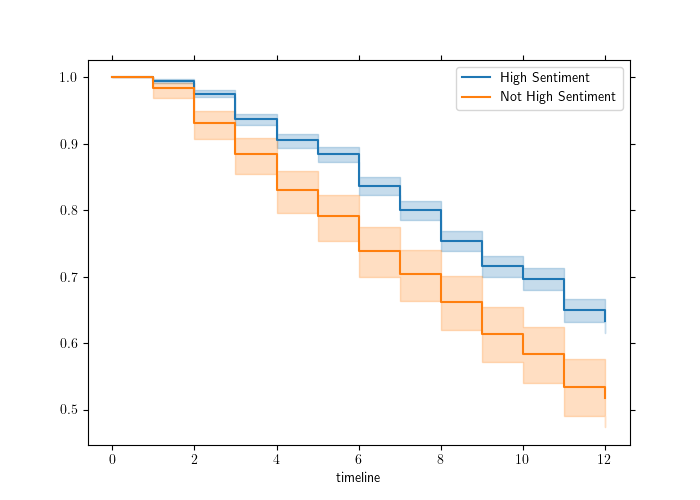
Figure 10.1: Survival curves by sentiment category in the job retention data
And here is an example of how to fit a Cox Proportional Hazard model similarly to Section 9.245.
from lifelines import CoxPHFitter

# fit Cox PH model to job_retention data
cph = CoxPHFitter()
cph.fit(job_retention, duration_col = 'month', event_col = 'left',
formula = "gender + field + level + sentiment")## <lifelines.CoxPHFitter: fitted with 3770 total observations, 2416 right-censored observations>
## duration col = 'month'
## event col = 'left'
## baseline estimation = breslow
## number of observations = 3770
## number of events observed = 1354
## partial log-likelihood = -10724.52
## time fit was run = 2025-01-20 14:39:00 UTC
##
## ---
## coef exp(coef) se(coef) coef lower 95% coef upper 95% exp(coef) lower 95% exp(coef) upper 95%
## covariate
## gender[T.M] -0.05 0.96 0.06 -0.16 0.07 0.85 1.07
## field[T.Finance] 0.22 1.25 0.07 0.09 0.35 1.10 1.43
## field[T.Health] 0.28 1.32 0.13 0.03 0.53 1.03 1.70
## field[T.Law] 0.11 1.11 0.15 -0.18 0.39 0.84 1.48
## field[T.Public/Government] 0.11 1.12 0.09 -0.06 0.29 0.94 1.34
## field[T.Sales/Marketing] 0.09 1.09 0.10 -0.11 0.29 0.89 1.33
## level[T.Low] 0.15 1.16 0.09 -0.03 0.32 0.97 1.38
## level[T.Medium] 0.18 1.19 0.10 -0.02 0.38 0.98 1.46
## sentiment -0.12 0.89 0.01 -0.14 -0.09 0.87 0.91
##
## cmp to z p -log2(p)
## covariate
## gender[T.M] 0.00 -0.77 0.44 1.19
## field[T.Finance] 0.00 3.34 <0.005 10.24
## field[T.Health] 0.00 2.16 0.03 5.02
## field[T.Law] 0.00 0.73 0.47 1.10
## field[T.Public/Government] 0.00 1.29 0.20 2.35
## field[T.Sales/Marketing] 0.00 0.86 0.39 1.36
## level[T.Low] 0.00 1.65 0.10 3.32
## level[T.Medium] 0.00 1.73 0.08 3.58
## sentiment 0.00 -8.41 <0.005 54.49
## ---
## Concordance = 0.58
## Partial AIC = 21467.04
## log-likelihood ratio test = 89.18 on 9 df
## -log2(p) of ll-ratio test = 48.58Proportional Hazard assumptions can be checked using the check_assumptions() method46.
## The ``p_value_threshold`` is set at 0.05. Even under the null hypothesis of no violations, some
## covariates will be below the threshold by chance. This is compounded when there are many covariates.
## Similarly, when there are lots of observations, even minor deviances from the proportional hazard
## assumption will be flagged.
##
## With that in mind, it's best to use a combination of statistical tests and visual tests to determine
## the most serious violations. Produce visual plots using ``check_assumptions(..., show_plots=True)``
## and looking for non-constant lines. See link [A] below for a full example.
##
## <lifelines.StatisticalResult: proportional_hazard_test>
##  null_distribution = chi squared
## degrees_of_freedom = 1
##              model = <lifelines.CoxPHFitter: fitted with 3770 total observations, 2416 right-censored observations>
##          test_name = proportional_hazard_test
##
## ---
##                                  test_statistic    p  -log2(p)
## field[T.Finance]           km              1.20 0.27      1.88
##                            rank            1.09 0.30      1.76
## field[T.Health]            km              4.27 0.04      4.69
##                            rank            4.10 0.04      4.54
## field[T.Law]               km              1.14 0.29      1.81
##                            rank            0.85 0.36      1.49
## field[T.Public/Government] km              1.92 0.17      2.59
##                            rank            1.87 0.17      2.54
## field[T.Sales/Marketing]   km              2.00 0.16      2.67
##                            rank            2.22 0.14      2.88
## gender[T.M]                km              0.41 0.52      0.94
##                            rank            0.39 0.53      0.91
## level[T.Low]               km              1.53 0.22      2.21
##                            rank            1.52 0.22      2.20
## level[T.Medium]            km              0.09 0.77      0.38
##                            rank            0.13 0.72      0.47
## sentiment                  km              2.78 0.10      3.39
##                            rank            2.32 0.13      2.97
##
##
## 1. Variable 'field[T.Health]' failed the non-proportional test: p-value is 0.0387.
##
##    Advice: with so few unique values (only 2), you can include `strata=['field[T.Health]', ...]` in
## the call in `.fit`. See documentation in link [E] below.
##
## ---
## [A]  https://lifelines.readthedocs.io/en/latest/jupyter_notebooks/Proportional%20hazard%20assumption.html
## [B]  https://lifelines.readthedocs.io/en/latest/jupyter_notebooks/Proportional%20hazard%20assumption.html#Bin-variable-and-stratify-on-it
## [C]  https://lifelines.readthedocs.io/en/latest/jupyter_notebooks/Proportional%20hazard%20assumption.html#Introduce-time-varying-covariates
## [D]  https://lifelines.readthedocs.io/en/latest/jupyter_notebooks/Proportional%20hazard%20assumption.html#Modify-the-functional-form
## [E]  https://lifelines.readthedocs.io/en/latest/jupyter_notebooks/Proportional%20hazard%20assumption.html#Stratification
##
## []
10.3 Inferential statistical modeling in Julia
The GLM package in Julia offers functions for a variety of elementary regression models. This package contains an implementation of linear regression as well as binomial logistic regression.
10.3.1 Ordinary Least Squares (OLS) linear regression
Here is how to run our OLS linear model on the ugtests data set from Chapter 4:
using DataFrames, CSV, GLM;

# get data
url = "http://peopleanalytics-regression-book.org/data/ugtests.csv";
ugtests = CSV.read(download(url), DataFrame);

# run linear model
ols_model = lm(@formula(Final ~ Yr1 + Yr2 + Yr3), ugtests)
## StatsModels.TableRegressionModel{LinearModel{GLM.LmResp{Vector{Float64}}, GLM.DensePredChol{Float64, CholeskyPivoted{Float64, Matrix{Float64}, Vector{Int64}}}}, Matrix{Float64}}
##
## Final ~ 1 + Yr1 + Yr2 + Yr3
##
## Coefficients:
## ───────────────────────────────────────────────────────────────────────────
## Coef. Std. Error t Pr(>|t|) Lower 95% Upper 95%
## ───────────────────────────────────────────────────────────────────────────
## (Intercept) 14.146 5.48006 2.58 0.0100 3.39187 24.9001
## Yr1 0.0760262 0.0653816 1.16 0.2452 -0.0522794 0.204332
## Yr2 0.431285 0.0325078 13.27 <1e-36 0.367492 0.495079
## Yr3 0.865681 0.0291375 29.71 <1e-99 0.808501 0.922861
## ───────────────────────────────────────────────────────────────────────────Summary statistics such as the \(R^2\) or adjusted \(R^2\) can be obtained using appropriate functions:
## 0.530327461953525## 0.528876362453896410.3.2 Binomial logistic regression
Here is how to run our binomial logistic regression on the salespeople data set from Chapter 5. Note that categorical inputs will need to be explicitly converted before running the model.
using DataFrames, CSV, GLM, Missings, CategoricalArrays;

# get salespeople data
url = "http://peopleanalytics-regression-book.org/data/salespeople.csv";
salespeople = CSV.read(download(url), DataFrame, missingstring=["NA"]);

# remove missing value rows from dataset
salespeople = salespeople[completecases(salespeople), :];

# ensure no missing data structures
salespeople = mapcols(col -> disallowmissing(col), salespeople);

# map categorical input columns
salespeople.performance = CategoricalArray(salespeople.performance);

# run binomial logistic regression model
promotion_model = glm(@formula(promoted ~ sales + customer_rate + performance), salespeople, Binomial(), LogitLink())
## StatsModels.TableRegressionModel{GeneralizedLinearModel{GLM.GlmResp{Vector{Float64}, Binomial{Float64}, LogitLink}, GLM.DensePredChol{Float64, CholeskyPivoted{Float64, Matrix{Float64}, Vector{Int64}}}}, Matrix{Float64}}
##
## promoted ~ 1 + sales + customer_rate + performance
##
## Coefficients:
## ──────────────────────────────────────────────────────────────────────────────────
## Coef. Std. Error z Pr(>|z|) Lower 95% Upper 95%
## ──────────────────────────────────────────────────────────────────────────────────
## (Intercept) -19.8589 3.44408 -5.77 <1e-08 -26.6092 -13.1087
## sales 0.0401242 0.00657643 6.10 <1e-08 0.0272347 0.0530138
## customer_rate -1.11213 0.482682 -2.30 0.0212 -2.05817 -0.166093
## performance: 2 0.263 1.02198 0.26 0.7969 -1.74004 2.26604
## performance: 3 0.684955 0.982167 0.70 0.4856 -1.24006 2.60997
## performance: 4 0.734493 1.07196 0.69 0.4932 -1.36652 2.8355
## ──────────────────────────────────────────────────────────────────────────────────The AIC, log likelihood and other summary statistics of the model can be obtained using the appropriate functions. For example:
## 76.3743282275113## -32.1871641137556510.3.3 Multinomial logistic regression
The Econometrics package provides a convenient function for a multinomial logistic regression model, where the levels of the outcome variable can be set as an argument.
using DataFrames, CSV, Econometrics, CategoricalArrays;

# get health_insurance data
url = "http://peopleanalytics-regression-book.org/data/health_insurance.csv";
health_insurance = CSV.read(download(url), DataFrame, missingstring=["NA"]);

# map gender and product to categorical
health_insurance.gender = CategoricalArray(health_insurance.gender);
health_insurance.product = CategoricalArray(health_insurance.product);

# fit model defining reference level
model = fit(EconometricModel,
            @formula(product ~ age + household + position_level + gender + absent),
            health_insurance,
            contrasts = Dict(:product => DummyCoding(base = "A")))
## Probability Model for Nominal Response
## Categories: A, B, C
## Number of observations: 1453
## Null Loglikelihood: -1595.27
## Loglikelihood: -744.68
## R-squared: 0.5332
## LR Test: 1701.18 ∼ χ²(12) ⟹ Pr > χ² = 0.0000
## Formula: product ~ 1 + age + household + position_level + gender + absent
## ───────────────────────────────────────────────────────────────────────────────────────────────────────
## PE SE t-value Pr > |t| 2.50% 97.50%
## ───────────────────────────────────────────────────────────────────────────────────────────────────────
## product: B ~ (Intercept) -4.60097 0.510551 -9.01179 <1e-18 -5.60248 -3.59947
## product: B ~ age 0.243662 0.0154313 15.7902 <1e-51 0.213392 0.273933
## product: B ~ household -0.967711 0.06943 -13.9379 <1e-40 -1.10391 -0.831516
## product: B ~ position_level -0.415304 0.0891671 -4.65759 <1e-05 -0.590215 -0.240392
## product: B ~ gender: Male -2.38258 0.232425 -10.251 <1e-23 -2.8385 -1.92665
## product: B ~ gender: Non-binary 0.252837 1.22625 0.206186 0.8367 -2.1526 2.65827
## product: B ~ absent 0.0116769 0.0129814 0.899512 0.3685 -0.0137875 0.0371413
## product: C ~ (Intercept) -10.2261 0.619736 -16.5007 <1e-55 -11.4418 -9.01041
## product: C ~ age 0.269812 0.0156702 17.2182 <1e-59 0.239073 0.300551
## product: C ~ household 0.204347 0.0496062 4.11938 <1e-04 0.107039 0.301655
## product: C ~ position_level -0.213592 0.0822607 -2.59652 0.0095 -0.374955 -0.052228
## product: C ~ gender: Male 0.0967029 0.195435 0.494809 0.6208 -0.286664 0.48007
## product: C ~ gender: Non-binary -1.26982 2.03625 -0.623608 0.5330 -5.26416 2.72452
## product: C ~ absent 0.00326628 0.0124181 0.263026 0.7926 -0.0210932 0.0276258
## ───────────────────────────────────────────────────────────────────────────────────────────────────────10.3.4 Proportional odds logistic regression
The Econometrics package also provides a convenient function for proportional odds logistic regression.
using DataFrames, CSV, Econometrics, CategoricalArrays;

# get soccer data
url = "http://peopleanalytics-regression-book.org/data/soccer.csv";
soccer = CSV.read(download(url), DataFrame, missingstring=["NA"]);

# map columns not starting with "n" to categorical
transform!(soccer, names(soccer, r"^(?!n)") .=> CategoricalArray, renamecols = false);

# map discipline column to ordinal
soccer.discipline = levels!(categorical(soccer.discipline, ordered = true), ["None", "Yellow", "Red"]);

# run proportional odds model
soccer_model = fit(EconometricModel,
                   @formula(discipline ~ n_yellow_25 + n_red_25 + position + result + country + level),
                   soccer)
## Probability Model for Ordinal Response
## Categories: None < Yellow < Red
## Number of observations: 2291
## Null Loglikelihood: -1915.63
## Loglikelihood: -1722.27
## R-squared: 0.1009
## LR Test: 386.73 ∼ χ²(8) ⟹ Pr > χ² = 0.0000
## Formula: discipline ~ n_yellow_25 + n_red_25 + position + result + country + level
## ─────────────────────────────────────────────────────────────────────────────────────────────
## PE SE t-value Pr > |t| 2.50% 97.50%
## ─────────────────────────────────────────────────────────────────────────────────────────────
## n_yellow_25 0.32236 0.0330776 9.74557 <1e-21 0.257495 0.387226
## n_red_25 0.383243 0.0405051 9.4616 <1e-20 0.303813 0.462674
## position: M 0.196847 0.116487 1.68986 0.0912 -0.0315846 0.425278
## position: S -0.685337 0.150112 -4.56551 <1e-05 -0.979707 -0.390967
## result: L 0.483032 0.111951 4.31466 <1e-04 0.263495 0.702569
## result: W -0.739473 0.121293 -6.09658 <1e-08 -0.977329 -0.501617
## country: Germany 0.132972 0.0935995 1.42065 0.1556 -0.0505771 0.316521
## level: 2 0.0909663 0.0935472 0.972411 0.3309 -0.09248 0.274413
## (Intercept): None | Yellow 2.50851 0.191826 13.077 <1e-37 2.13234 2.88468
## (Intercept): Yellow | Red 3.92572 0.205714 19.0834 <1e-74 3.52232 4.32913
## ─────────────────────────────────────────────────────────────────────────────────────────────Note that the \(R^2\) results presented correspond to the McFadden variant of the pseudo-\(R^2\), although other variants can be obtained by specifying them in the appropriate function.
## 0.1912444622950184910.3.5 Mixed models
The MixedModels package allows for the construction of both linear mixed models and mixed GLMs. Here is an approach to our mixed model on speed dating from Section 8.1:
using DataFrames, CSV, MixedModels, CategoricalArrays;

# get speed_dating data
url = "http://peopleanalytics-regression-book.org/data/speed_dating.csv";
speed_dating = CSV.read(download(url), DataFrame, missingstring=["NA"]);

# make iid categorical
speed_dating.iid = CategoricalArray(speed_dating.iid);

# run mixed GLM
dating_model = fit(MixedModel, @formula(dec ~ agediff + samerace + attr + intel + prob + (1|iid)),
                   speed_dating, Binomial(), LogitLink())
## Generalized Linear Mixed Model fit by maximum likelihood (nAGQ = 1)
## dec ~ 1 + agediff + samerace + attr + intel + prob + (1 | iid)
## Distribution: Bernoulli{Float64}
## Link: LogitLink()
##
## logLik deviance AIC AICc BIC
## -3203.2192 6406.4385 6420.4385 6420.4529 6469.1617
##
## Variance components:
## Column VarianceStd.Dev.
## iid (Intercept) 5.15260 2.26993
##
## Number of obs: 7789; levels of grouping factors: 541
##
## Fixed-effects parameters:
## ──────────────────────────────────────────────────────
## Coef. Std. Error z Pr(>|z|)
## ──────────────────────────────────────────────────────
## (Intercept) -12.7909 0.370179 -34.55 <1e-99
## agediff -0.0369841 0.0138019 -2.68 0.0074
## samerace 0.203861 0.0800888 2.55 0.0109
## attr 1.07878 0.0307969 35.03 <1e-99
## intel 0.302556 0.033378 9.06 <1e-18
## prob 0.620642 0.0267356 23.21 <1e-99
## ──────────────────────────────────────────────────────